Most of our examples contain a common set of "beginning" commands as well as a common "ending" command. Click here to get documentation for these commands. They will not be discussed directly. The files which are discussed here are:
If you look at the new data file, you will notice that four new commands have been added:
     &DESCRIBE LOAD_GROUP CARGO
     *CAR_CG 90 0 20
     #WEIGHT *CAR_CG 1000 16 16 20
     #AREA *CAR_CG 50*20 0     0
     #AREA *CAR_CG 0     50*20 0
The first of these commands defines a "LOAD GROUP" with a name of CARGO.
A load group is a MOSES abstraction. Simply speaking, it is a set of
load attributes given a name and an associated set of nodes.
Normally, one also needs to define a set of nodes with each load group.
These nodes will receive the loads created by the group in any structural
analysis. Here we did not define any nodes. For this stage of our transportation
analysis we are not interested in specifying a node map. Later, when we
perform a structural analysis we will be interested in mapping the load to
the proper nodes. So what does the program do when it expects a selector,
and none is provided? The program will select all available nodes.
There will be more about nodes and load mapping in a later section.
The command "*CAR_CG 90 0 20" defines a "point" that is located at x = 90, y = 0, and z = 20 feet from the vessel origin. This will be used to define the center of gravity and the centroid of the wind area for the cargo loadgroup. The #WEIGHT which follows defines the weight of the group. This command instructs MOSES that a weight of 1000 kips is attached to the vessel at the location of *CAR_CG. This weight has radii of gyration of 16, 16 and 20 about the x, y and z axes respectively. To learn more about the #weight command click here.
The next two lines use the command #AREA. This command defines a wind for the cargo. The center of the area is at the *CAR_CG location. The size of the area is 50*20 ft^2. The first line defines the area to be used when computing the x-direction component and the second line defines the area to be used when computing the y-direction component. We have chosen to use #AREA for the cargo because we do not expect the cargo to enter the water at any point during the analysis. To learn more about the #AREA command click here.
Now let us turn to the cif file.
If you look at the command file, you will notice that there are not many new commands. Stability is again computed, but the most important change is the addition of the command:
&APPLY -LOAD_GROUP -PERCENT CARGO 100
Even though we have defined the cargo, it will not alter the answers
unless it is "applied". The above command says to apply the CARGO
load group with a percentage of 100.
Again, we create the vessel plots. When you view these, you will notice that they have not changed (load groups do not register). We have not told it the dimensions of the cargo, only the center of gravity. When we discuss the methods of adding cargo, we will talk about how cargo can be viewed in plots.
After the plots we ballast the vessel. If you look at the log, you will notice that the ballast arrangement for this analysis is different than the previous analyses we have performed. The difference in the ballast arrangement arises from the weight of the cargo that was added. Now that we have added 1000 Kips of cargo, we have taken away some water from the ballast arrangement to achieve equilibrium. The ballast water in this analysis weighs 2569 Kips in comparison to the previous weight of 2712 Kips in the file rao.ans/log00001.txt. The difference between 2712 and 2569 is not 1000 Kips, but 142 Kips because we are now at a deeper draft and a higher trim angle. The addition of cargo and the new ballast arrangement has also changed the center of gravity of the system and the radii of gyration. All of these changes will be evident in the stability results and RAOs.
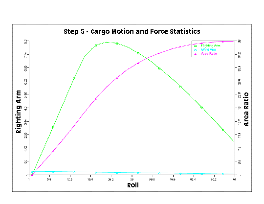
In the stability analysis, results in the output file show a noticeable change in the area ratio. At a 10 degree roll, we had 28.3 kips-ft. Now at 10.5 we have 10.6 kips-ft. In this run, we have added a plot of the righting arm results. The command we have used is:
PLOT 2 5 7 -RAX 9 -NO
This command is in the Disposition menu under the Hstatic menu. We instruct the
program to create a plot with the values in column 1 as the abscissa. On the
ordinate on the left hand side, plot columns 5 and 7. On the ordinate on the
right hand side, plot column 9. At the end of this command we have used the
option -NO. This options instructs the
program that we do not want to answer questions concerning the titles and
legends to use on the plot.
(For details, click here.)

In the RAOs we also see changes. The changes start from the locations which RAOs are reported. In the com file, we instructed the program to report RAOs at the system CG. The location of the CG has changed with the addition of the cargo, and with the change in CG comes changes in RAOs.
As you can see the addition of cargo is a very essential step. Now that we have added cargo, established a new ballast arrangement, performed a stability analysis and calculated the RAOs, we need to find forces and accelerations for the transportation. We have the first ingredient needed to calculate forces and accelerations, the RAOs. Now we need an environment description. With the environment description we then will be able to perform a spectral analysis.
