Although the float-off presented here is basic, the concepts that are introduced are fundamental for any float-off analysis. This sample contains a macro to make the flooding reports during the flooding sequence uniform. The post processing is meant to show a procedure that could be copied to other float-offs. It is not meant to be inclusive of all possible post processing options.
Most of our examples contain a common set of "beginning" commands as well as a common "ending" command. Click here to get documentation for these commands. They will not be discussed directly. The files which are discussed here are:
- the main data file
- amt barge plus some modifications
- the buoy model
- basic float-off commands
- basic float-off log
There are five major parts to the analysis:
- Define the two bodies (the barge and buoy model)
- Put the two bodies in the starting positions (the buoy on top of the barge )
- Make the compression only connections between the two bodies
- Flood the compartments in a pre-designed order
- Generate the results
The two bodies are defined in the dat file float.dat. The file float.dat reads in the files barge.dat and buoy.dat.
Here is the text of the float.dat file.
$
$   READ BARGE MODEL
&insert ./barge.dat
$
$   READ BUOY  MODEL
&insert ./buoy.dat
The file is fairly simple. It reads in the barge and the buoy model This is the first tutorial where there is a secondary set of data files for the models. Reviewing the file barge.dat, we find it contains two sections. The first section which reads in the AMT_CARR barge then makes some changes. All of the buoy description is contained in the buoy.dat file. files.
In the float.dat we insert the barge and buoy models using the command &insert. The &insert command is handy when there are several files involved. For the projects that have many bodies, or the bodies have many pieces sometimes it is advantageous to keep track of all the information in separate files.
Here is the text of the barge model.
$
$ Model information files
$
&dimen -save -dimen meters m-tons
use_ves amt_carr
&describe body amt_carr
$
$ ******************************      points needed for draft marks
$
*bpt 0 -13.716 6.096
*bpb 0 -13.716 0
*bst 0 13.716 6.096
*bsb 0 13.716 0
*spt 91.35 -13.716 6.096
*spb 91.35 -13.716 0
*sst 91.35 13.716 6.096
*ssb 91.35 13.716 0
$
$ ******************************      define draft marks
$
&describe body amt_carr -dmark bp *bpb *bpt \
	-dmark bs *bsb *bst \
	-dmark sp *spb *spt \
	-dmark ss *ssb *sst \
		-section 1.66e8 45 2.40 \
		-location 0 5 10 15 20 25 30 35 40 45 50 55 60 \
				65 70 75 80 85 90 91.35
$
$ ******************************      points needed for connectors
$
*b1 2*8.22   0  6.096
*b2 8.22     0  6.096
*b3 0        0  6.096
*b4 8.22  -8.22 6.096
*b5 8.22   8.22 6.096
$
&dimen -rem
First we are using the AMT_CARR barge from the barge library. To this barge we are adding draft marks and some points to be used for the connectors. Notice that to define the draft marks, you must first define the points that will be used on the &describe body command to define the draft marks. Also, it is necessary to have at least two &describe body commands to define draft marks. In this file we only see the second and third occurrence of &describe body. The first occurrence is within the vessel file in the vessel library.
We are defining four draft marks, bp - bow port, bs - bow starboard, sp - stern port, and ss stern starboard. It is necessary for there to be an option -dmark for each separate draft mark. Also, it is necessary for the order of the points to be bottom to top. If you reverse the order MOSES will be reporting freeboard.
In the last section pertaining to the AMT_CARR barge we define five points that will later be used in the cif file. These points can be defined either in the dat file or in the cif file. This concludes the barge file.
The buoy is the second body read in by the float.dat file. Here is the buoy.dat file.
$
$
$****************************************          Set Dimensions
$
&dimen -save -dimen Meters   M-Tons
&LOCAL xfac = 1 yfac = 1 zfac = 1
$
$****************************************          Defaults
$
&model_def -save
&model_def -fyield 248.04 -alpha 3.6111E-6 -spgravit 7.8492 -emodulus \
       1.9981E5 -poi_ratio 0.3 -kfac 1 1 -cmfac 0.85 0.85 -flood no -use @
$
$
$****************************************          Set body to buoy
$
&describe body buoy
$
$****************************************          Define Points
*f1  8.22   0 0
*f2  0      0 0
*f3 -8.22   0 0
*f4  0  -8.22 0
*f5  0   8.22 0
*bcg 0    0 7.354
#weight *bcg 500 27.4 27.4 5.5  -cat Buoy
$
$****************************************          Define Buoy Shape
$
$
pgen buoy -loc 0  0  0  0 -90
   plane 0  10 -circ  0 0 8.22 0 10 18
end_pgen
&dimen -rem
As you can see the buoy file is really a simple description of a cylindrical shape. The file has two sections. The first section defines the body buoy and the points to be used in the cif file for the connectors, and a weight. The second part describes the outer shell of the buoy.
That completes the discussion on the data files. We now proceed to the command input (cif) files.
Put the two bodies in the starting position
We use the common commands to read in the vessel and the buoy model. Then we position the two bodies with the following commands.
$
$ ****************************  set variable for barge draft
$
&set h_amt = 4.27
$
$ ****************************  start at even keel
$
&instate -draft sp %h_amt  bp %h_amt bs %h_amt ss %h_amt
$
$ ****************************  set height of buoy (distance from barge deck)
$
&set h_buoy = &number(real %(vdepth)-%h_amt+1.00)
$
$ ****************************  place buoy
$
&instate -move buoy 8.22 0 %h_buoy
The barge position is done first with two commands. In the first command, the variable h_amt is set to 4.27, then by using the command &instate -draft the barge is set at even keel.
It might seem extraneous to have a variable specifically for the barge draft. Here we need to use it, h_amt, twice: once to set the barge draft and again to locate the buoy at the correct height above the barge deck.
For the placement of the buoy we have several things to keep in mind.
- In the dat file we have described the buoy as a body.
- In the dat file we defined the buoy body coordinate system to have a z = 0 at the bottom of the buoy.
- The body location is set with reference to the global coordinate system.
- We want to set the buoy 1 meter above the barge deck.
Just as we did for the barge we place the buoy in the global coordinate system with the &instate command. When we placed the barge we used the -draft option, here we use the -move option. (Please click here for the manual page on &instate.)
The next two sets of commands are set off by comments which read: "find length between buoy and barge" and "report spring end locations". These two sections are there to first check our work and second to make sure the bodies are positioned correctly for the connectors.
$
$ ****************************  find length between buoy and barge
$
&set c_len = &point(d_node *f1 *b1)
$
$ ****************************  report spring end locations
$
&type f1 &point(coord *f1 -g) b1 &point(coord *b1 -g)
&type f2 &point(coord *f2 -g) b2 &point(coord *b2 -g)
&type f3 &point(coord *f3 -g) b3 &point(coord *b3 -g)
&type f4 &point(coord *f4 -g) b4 &point(coord *b4 -g)
&type f5 &point(coord *f5 -g) b5 &point(coord *b5 -g)
$
$ ****************************  get picture
$
&picture starb
Here we are using the string function &point to verify the distance between the barge and the buoy. (Please click here for the manual page on &point.) We are also saving the length between the two to the variable "c_len". This variable will later be used for the connectors. In the set beginning with the command &type we are reporting the location in the global coordinate system of the two attachment points for the connectors.
If you look at the results in the log file you will see that MOSES has substituted the x, y, and z location of each point for the command &point(coord *name -g). Here is an excerpt from the log file.
 f1 16.44 0 2.82 b1 16.44 0 1.826
 f2 8.220001 0 2.82 b2 8.220001 0 1.826
 f3 0 0 2.82 b3 0 0 1.826
 f4 8.220001 -8.220001 2.82 b4 8.220001 -8.220001 1.826
 f5 8.220001 8.220001 2.82 b5 8.220001 8.220001 1.826
As you can see the points on the barge are directly below the points of the buoy. For all five sets the z location changes by 1 meter. The only change is in the third decimal place. This difference is not large enough to change our assumptions.
For a float-off we want to define compression only connectors. And we want them to start with a total force equal to the weight of the buoy. This will be checked after the connectors have been defined. The point in these two small sections is to provide a check on the distance between the buoy and the barge. We need to know the distance between each set of connectors to assure ourselves there is no unintended rotation, compression, or tension.
Since this is a multi body system it is good practice to put in checks on our work. This step is a check of our work and allows us to verify that the set up is correct. This checking step in general is not needed for the analysis to continue.
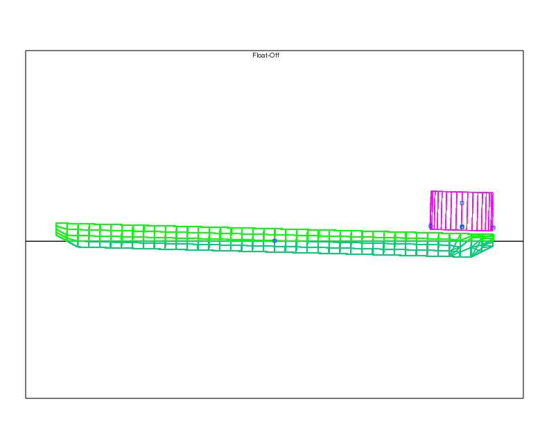
At the end of this section we produce a picture of the set up, so far.
Make the compression only connections between the two bodies
The next section is where the connectors are described. The connectors description and modeling is all done within the model editing menu. This section begins with the command medit and ends with the command end_medit. (Please click here for the manual page on medit.)
$
$ ****************************  make connection between buoy and barge
$
medit
$
$ ****************************  make spring stiff only in x direction
$
  ~conn gspr compression x 1e3 1e3 y 1e1 1e1 z 1e1 1e1 \
         rx 1e1 1e1 ry 1e1 1e1 rz 1e1 1e1  -len %c_len
$
$ ****************************  stiffness should be up and down (+z)
$
   connector c1 ~conn -euler +z  *b1 *f1
   connector c2 ~conn -euler +z  *b2 *f2
   connector c3 ~conn -euler +z  *b3 *f3
   connector c4 ~conn -euler +z  *b4 *f4
   connector c5 ~conn -euler +z  *b5 *f5
end_medit
The properties of the connector class are described with the command
that begins ~conn. Here only the character ~ is the command,
however, the connector name is "~conn".
(Please
click here for
the manual page on ~.)
We are defining a connector that has a stiffness in the x element direction
of 1e3 m-tons/m and a stiffness in the y and z element directions of 1e1 m-tons/m.
The rotational stiffness has also been set to 1e1 m-ton m / degree. If you are
not sure of the units MOSES is using please
click here for
the manual page on dimensions. The last property we designate is the "nominal"
length, with -len. For our float-off analysis this would be the
unstreched/uncompressed length where the connector is activated.
Now that we have the connector properties we can define the connectors. This is done with the command connector. (Please click here for the manual page on connector.) To define the connectors we give them a name (for example "c1"), properties (associated with "~conn"), change the connector ("element") system so that the element x axis is parallel to the barge z body axis ("-euler +z") and we designate the two nodes to connect (*b1 *f1). Most of these properties seem straight forward. The orientation of the element x axis is the one that seems to be missed most often. What we are modeling here is the buoy sitting on stiff supports. We are making the assumption that all the sea-fastenings have been removed so there is very little stiffness in the transverse or longitudinal direction. We want the connectors to be stiff in the barge z direction and weak in the other directions. This is why we change the element x-axis to be parallel to the body z-axis.
This concludes the connector definitions, with the command end_medit.
In the next section we write a macro. You can think of it as making a new MOSES command. The purpose of this command is to find an equilibrium position, make a set of reports and create a picture. The macro definition begins with the command ¯o and ends with the command &endmacro. (Please click here for the manual page on macros.) The section of the cif file that defines the macros is:
$
$ **************************** make a macro for repositioning
$
¯o new_pos -amount p_arg pair
&if %p_arg &then
&set n_comp = &token(n %pair)
&set s_comp = &number(integer %n_comp/2)
&loop c_bal 1 %n_comp 2
&set b_name = &token(%c_bal %pair)
&set b_per = &token(1+%c_bal %pair)
&compart -amount %b_name %b_per
&endloop
&endif
&equi -maxit 1000
&event %i
&subtitle Event %i
&type Event %i
&set i = &number(integer 1+%i)
&status config
&status f_connect
&picture starb
&status force
&status f_conn
&status compart
&endmacro
&set i = 0
Most of the commands used in the macro have been discussed in
the
stability discussion or
the
sea keeping discussion. Therefore the macro will not be
discussed in detail here. The command that is used several times
is &status, you can
click here to read on all the options available with the command.
Most of the commands in the next section should be familiar. What may not be familiar is the results. The tables produce with the &status commands now have a section for each body. Here is an example of the MOSES window when it is reporting the status reports for configuration and force.
What we want to pay special attention to is that for the barge report there is a large moment about the y axis (MY = -39024 m-tons). Up to this point we have placed the buoy near the bow end of the barge and we have added weight in the compartments by added ballast. This moment means that when we ask MOSES to find an equilibrium position, the equilibrium position will have a trim.
The next set of commands that are new to the tutorial section, is the &describe body -ignore. When MOSES is asked to find equilibrium MOSES will normally look at all six degrees of freedom. If you review the results of the &status force command you will notice that there is moment about the X and Y body axis of the AMT_CARR barge. When MOSES is asked to find the equilibrium position we are asking MOSES to change the condition such that we are near the sum of the forces equal zero and the sum of the moments equal zero. we want MOSES to correct the roll and pitch of the barge without changing the X, Y, and RZ position much. If we do not somehow tell MOSES this, MOSES will change X, Y, and RZ as part of trying to reposition RX and RY. With the command &describe body -ignore we telling MOSES to ignore forces in the X and Y direction when solving the force equations, and to ignore the moment about the Y axis when solving the moment equations. Please click here for the manual page on &describe body -ignore. This next set of commands are commented as "find equilibrium to start".
$
$ ****************************  no moorings so do not move in x-y plane
$
&describe body amt_carr  -ignore x y
$
$ ****************************  buoy does not yaw
$
&describe body buoy      -ignore x y rz
$
$ ****************************  find equilibrium to start
$
&status force
&equi -maxit 1000
&status force
$
$ ****************************  draft marks - where are they?
$
&status draft
$
$ ****************************  forces on the connectors
$
&status f_connect
If we review the new configuration and forces we see that the force totals are very near zero, and that the equilibrium position does have a trim. We also notice that the equilibrium position did not change the degrees of freedom we asked MOSES to ignore. Here is an excerpt from the log file.
The next section, commented as "draft marks - where are they?", is there for us to check our work. During the larger projects there are many departments involved, and many times it is advantageous to be able to confirm some of the basic parameters. Here we are confirming the draft marks readings. The readings show that there is a 2.4 m trim by the bow (please see the log file). That is the bow draft readings (BS BP) are 2.4 m deeper than those at the stern (SS SP).
In the next report, commented as "forces on the connectors" we see that the weight of the buoy is almost evenly distributed. We see that connector C3 being closer to the bow does take more weight, in comparison to connector C1 which is furthest from the bow. This stands to reason since our barge has a trim by the bow. In the next section we again check the connector end locations, and we create a picture of the configuration before the ballast sequence.
$
$ ****************************  check on spring end locations
$
&type *********************************************
&type f1 &point(coord *f1 -g) b1 &point(coord *b1 -g)
&type f2 &point(coord *f2 -g) b2 &point(coord *b2 -g)
&type f3 &point(coord *f3 -g) b3 &point(coord *b3 -g)
&type f4 &point(coord *f4 -g) b4 &point(coord *b4 -g)
&type f5 &point(coord *f5 -g) b5 &point(coord *b5 -g)
&type *********************************************
$
$ ****************************  make picture for starting stage
$
&subtitle Before Ballast Sequence
&picture starb
Just like we did earlier, this is to check that the connectors are representing the supports that we are trying to model. Here we are checking that the distance between the two ends is one meter. As we see, the connectors are still good and we can now proceed with the flooding sequence.
Flood the compartments in a pre-designed order
So far, we have made a picture of our current position. Now we want to report and define this position as event 1. We do this by running our macro "new_pos". From this point forward the flooding sequence begins and all we do is tell MOSES what ballast to add when we call our macro. The ballast sequence is commented by "flooding sequence simulation" and "end of flooding" and is shown below.
$
$ ****************************  make basic reports for starting stage
$
new_pos
$
$ ****************************  flooding sequence simulation
$
new_pos -amount 1p 324 1s 324
$
new_pos -amount 1c 756 1p 405 1s 405
$
new_pos -amount 1c 810 1p 435 1s 435 2p 587 2s 587
$
new_pos -amount 2c 461
$
new_pos -amount 2c 923
$
new_pos -amount 3c 462
$
new_pos -amount 3c 923
$
new_pos -amount 5p 88 5s 88
$
new_pos -amount 5p 118 5s 118
$
$ ****************************  end of flooding
$
What makes this section look so clean is the use of our macro. The only thing we are changing between each step is the ballast condition. Our macro, new_pos finds a new equilibrium position and creates the four reports and a picture.
Generate results
Now that we have run the analysis, we need to view the results. We do this using the prcpost command. This section is commented by "begin post processing". The prcpost command enters us into the post processing menu. We know that we are in the Post Processing menu because the MOSES window frame now shows "MOSES - PROCESS POST-PROCESSING" on the top bar. An example is shown below.
It is worth noting that the commands in the Post Processing Menu would be applicable to any analysis that has events. For our simple float off there are only nine events. For a motions analysis done in the time domain there can be thousands of events.
Here we reported some quantities that were of interest to our particular project. There are many more quantities that are available for reporting. The purpose of presenting the post processing particular to this project is to show an example of how the commands work. With this set of commands you should be able to process many of the other quantities.
The post processing section is divided into three sections: connector forces, trajectories, and ballasting. The post processing section is shown below.
$ ****************************  begin post processing
$
prcpost
$
$ ****************************  report connector forces
$
   conforce
      vlist
      plot 1 8 16 24 32 40 -no
      statistic 1 8 16
      extreme   1 24 32 40
   end
$
$ ****************************  report trajectories (motion)
   trajectory
      vlist
      plot 1 4 -rax 7 -no
      plot 1 8 9 -no
      view 1 8 9
   end
$
$ ****************************  report ballasting
   tank_bal
      vlist
      plot 1 66 -rax 115 122 -no
      extreme 1 115 122
   end
end
If you look at the three sections for post process you will see that there
are three commands vlist, plot, and end
that are common to all the sections. Basically the commands:
     vlist gives us a list of the available variable,
     plot produces a plot of some of the variables,
     end return to the post processing menu.
For each entrance into a sub-menu a different command is used. The command
depends on what quantities are of interest.
For the first set we are interesting in connector forces, conforce.
When we review the log file we see the results of the vlist command to be:
                  The Variables Available for Selection are:
                  ==========================================
   1 Event                  15 MZ:C2                    29 MX:C4
   2 FX:C1                  16 MAG:C2                   30 MY:C4
   3 FY:C1                  17 M/BT:C2                  31 MZ:C4
   4 FZ:C1                  18 FX:C3                    32 MAG:C4
   5 MX:C1                  19 FY:C3                    33 M/BT:C4
   6 MY:C1                  20 FZ:C3                    34 FX:C5
   7 MZ:C1                  21 MX:C3                    35 FY:C5
   8 MAG:C1                 22 MY:C3                    36 FZ:C5
   9 M/BT:C1                23 MZ:C3                    37 MX:C5
  10 FX:C2                  24 MAG:C3                   38 MY:C5
  11 FY:C2                  25 M/BT:C3                  39 MZ:C5
  12 FZ:C2                  26 FX:C4                    40 MAG:C5
  13 MX:C2                  27 FY:C4                    41 M/BT:C5
  14 MY:C2                  28 FZ:C4
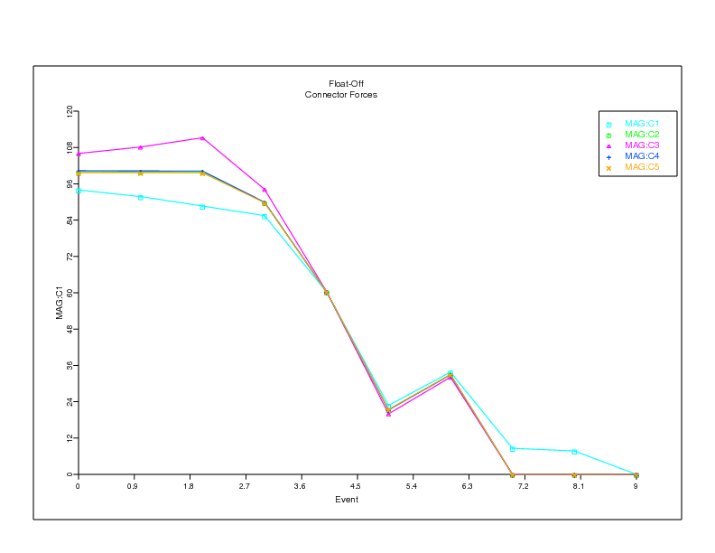
When we asked for a plot of "1 8 16 24 32 40" we were asking for a plot of event vs
magnitude of each separate connector. The results of vlist map the numbers
in the plot command to the variables. So 1 is Events, 8 is MAG:C1 or the magnitude
of connector C1, and so forth. The option -no stands for "no changes".
If you take this option out MOSES will ask you about possible changes. Here you are
starting by telling MOSES that you do not want changes. Here is the first results
of the first plot command.
In the next command extreme 1 24 34 40 we ask for the extremes of the magnitude of connectors C3, C4, and C5. Again, these numbers would be more exciting if the analysis had been done in waves and had more events.
Then we end out of the Connector Force sub-menu with the command end and this places us back into the Post Processing menu.
For the section beginning with the command trajectory we are interested in the trajectories, or motions, of the two bodies. The command trajectory enters us into the Trajectory sub-menu. Just as before there is an end a few lines down so that we exit the Trajectory sub-menu and are placed back in the Post Processing menu. Please click here for the manual page on trajectory command and sub-menu.
Just as with the connector data here we us the commands vlist and plot to view the available variables. The new command here view lets us look at the values of three of the variables 1 - Event, 8 - RX:AMT_CARR, and 0 - RY:AMT_CARR. The command view presents the values in tabular form instead of graphic form as with the command plot.
The last section begins with the command tank_bal in which we look at the ballast in the compartments. Here we use the same set of commands to look at variable pertinent to compartment ballast. Here the mapping of the variables with the numbers is reported, and there is a plot, and an extreme report.
At the end of this section there is an end to return us to the Post Processing menu and there is an end to get us back to the Main Menu. Finally at the end we create a movie of our float-off and finish the simulation.
$
$ ****************************  make a movie
$
&subtitle
&picture starb -movie mpg  1 1 -render gl -event 0 9 1
&fini